Mathematical Models

To understand what models are actually doing we need to utilise mathematical models. The concept was popularised in the late 60’s by Don Knuth.

We can calculate the total running time of an operation with the below mathematical model.

sum of cost x frequency of all operations

Analyse program to determine set of operations.
Cost depends on machine, compiler.
Frequency depends on algorithm, input data.

Cost of basic operations

Today we run experiments to understand the cost of operations. As an example we could run an add operation a billion times to average the time in nano seconds to run that operation, below are types of operations to consider:

int add
int multiply
int divide
float add
float multiply
float divide
sine
arctangent
var declaration
assignment statement
array element access
1d array allocation
2d array allocation
string length
substring extraction
string concat

It is important to understand the operation itself and how that could effect running time for example string concatenation is proportional to the length of the string so this could change the running time of the operation significantly

The sum of these basic operations present in our algorithm will be used as our first component in our mathematical model.

Example: 1-Sum

int count = 0;
for(int i = 0; i < N; i++){
  if(a[i] == 0){
    count++;
  }
}

Operations to consider and frequency

variable declaration = 2
assignment statement = 2
less than compare = N + 1
equal to compare = N
array access = N
increment = N to 2 N

Example: 2-Sum

int count = 0;
for (int i = 0; i < N; i++){
  for(int j = 0; j < N; j++){
    if(a[i] + a[j] == 0){
      count++;
    }
  }
}

Operations to consider and frequency

We have exponentially increased the frequency of our operations within the brute force method.

variable declaration = N + 2
assignment statement = N + 2
less than compare = $\frac{1}{2} (N+ 1) * (N + 2)$
equal to compare = $\frac{1}{2} N * (N - 1)$
array access = $N * (N - 1)$
increment = $\frac{1}{2} N * (N - 1) to N * (N - 1)$

It is convenient to have a measure of the amount of work involved in a computing process, even though it be a very crude one. We may count up the number of times that various elementary operations are applied in the whole process and then given them various weights. We might, for instance, count the number of additions, subtractions, multiplications, divisions, recording of numbers, and extractions of figures from tables. In the case of computing with matrices most of the work consists of multiplications and writing down numbers, and we shall therefore only attempt to count the number of multiplications and recordings.

Alan Turing (Rounding-Off Errors in Matrix Processes)

To paraphrase based on Turing’s suggestions we weight our operations by most expensive and count the frequency of those which are most expensive or executed most often as a proxy for running time. Essentially we hypothesize our running time utilising this method.

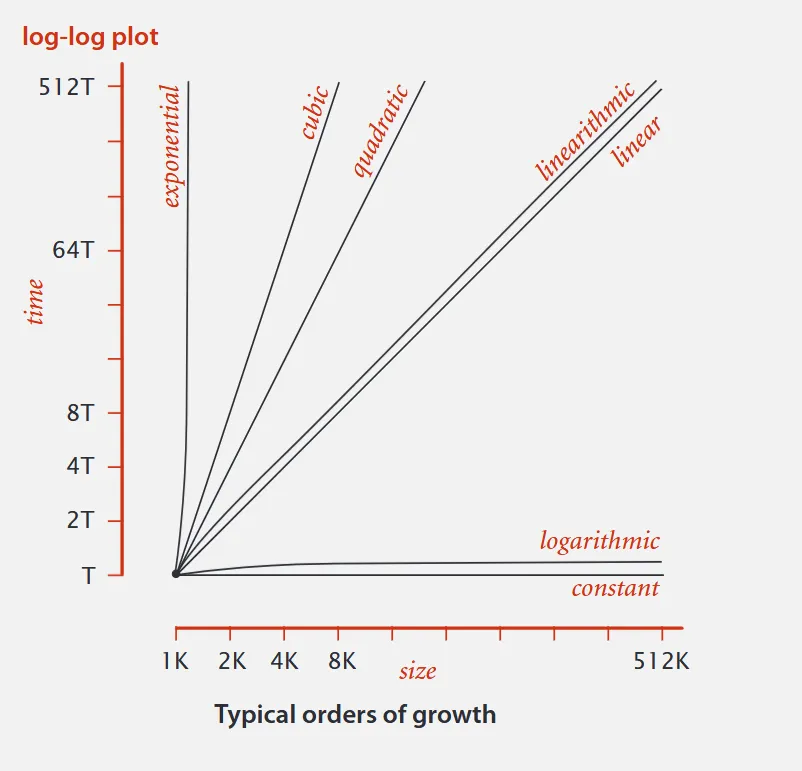
Only a few functions really turn up when we analyse algorithms. A great number of algorithms are described by these few functions:

$\log(n)$
$N$
$N \log N$
$N^2$
$N^3$
$2^N$

table of growth When we talk about order of growth we discard the leading coefficient as an example if we hypothesize the running time of an Algorithm is $N \log N$ what that actually means is the running time of an algorithm is $CN \log N$ where C is some constant.

Common order-of-growth classifications

Order of Growth	Name	Typical Code Framework	Description	Example	T(n)T(2n)
$1$	Constant	`a = b + c`	Statement	Add two numbers	$1$
$\log N$	Logarithmic	`while(N > 1) N = N/2`	Divide in half	Binary search	$\approx 1$
$N$	Linear	`for (int i = 0; i < N; i++)`	Loop	Find the maximum	$2$
$N \log N$	Linearithmic	(See mergesort)	Divide and conquer	Mergesort	$\approx 2$
$N^2$	Quadratic	`for(..){for(..)}`	Double loop	Check all pairs	$4$
$N^3$	Cubic	`for(..){for(..){for(..)}}`	Triple loop	Check all triples	$8$
$2^N$	Exponential	(See combinatorial search)	Exhaustive search	Check all subsets	$T(n)$

Problem Size solvable in minutes

Growth Rate	1970s	1980s	1990s	2000s
$1$	Any	Any	Any	Any
$\log N$	Any	Any	Any	Any
$N$	Millions	Tens of Millions	Hundreds of Millions	Billions
$N \log N$	Hundreds of Thousands	Millions	Tens of Millions	Hundreds of Millions
$N^2$	Hundreds	Thousands	Thousands	Tens of Thousands
$N^3$	Hundreds	Hundreds	Thousands	Thousands
$2^N$	$\approx 20$	$20s$	$20s$	$\approx 20$

Conclusion We need linear algorithms to keep pace with Moore’s law.

Notation

One way to simplify our analysis of an algorithm employing mathematical methods is to use tilde notation. Tilde notation works of the two core principles.

Estimate running time (or memory) as a function of input size N.
Ignore lower order terms.
- When N is large, terms are negligible.
- when N is small, we don’t care.

Example 1:	$\frac{1}{6} N^3 + 20N + 16$	~ $\frac{1}{6}N^3$
Example 2:	$\frac{1}{6} N^3 + 100 N^\frac{4}{3} + 56$	~ $\frac{1}{6}N^3$
Example 3:	$\frac{1}{6}N^3 + \frac{1}{2} N^2 + 1/3N$	~ $\frac{1}{6}N^3$

To surmise:

In principle: Accurate Mathematical Models are available.
In Practice:
- Formulas can be complicated.
- Advanced mathematics might be required.
- Exact models best left for the experts.

To summarise our analysis of an algorithm there are a couple of commonly used notations to help describe our order of growth.

notation	provides	example	shorthand for	used to
Big Theta	asymptotic order of growth	$Θ(N^{2})$	$\frac{1}{2} N^{2}$ $10 N^{2}$ $5 N^{2} + 22 N log N + 3N$	classify algorithms
Big Oh	$Θ(N^{2})$ and smaller	$O(N^{2})$	$10 N^{2}$ $100 N$ $22 N log N + 3 N$	develop upper bounds
Big Omega	$Θ(N^{2})$ and larger	$Ω(N^{2})$	$\frac{1}{2} N^{2}$ $N^{5}$ $N^{3} + 22 N log N + 3 N$	Develop Lower Bounds